Power and Data Rate Assignment
for Maximal Weighted Throughput:
A Dual-Class 3G CDMA Scenario

Virgilio Rodriguez, David J. Goodman
Polytechnic University
ECE Department
5 Metrotech Center
Brooklyn, NY 11201

Abstract

1  Introduction

Modern wireless networks will accommodate simultaneous transceivers operating at very different bit rates. Several technologies have been proposed to accommodate multi-rate traffic in such networks. Ottosson and Svensson [3] discuss several multi-rate schemes based on Direct Sequence Code-Division Multiple Access (DS-CDMA). One such scheme is variable spreading gain (VSG) CDMA, as described, for example, by I and Sabnani[1]. In a VSG-CDMA system, each terminal's spreading gain is defined as the ratio of the common chip rate to the terminal's bit rate.

Our model is relevant to an interference-limited single-cell VSG-CDMA system in which each data terminal can operate within a range of bit rates, assumed continuous for tractability. We seek allocations of data rate and power levels which will maximize the network weighted throughput. There are two possible weights, which admit various interpretations, including levels of importance or priority, ``utilities'', or monetary prices. We assume the traffic to be delay-tolerant.

Two recent publications of ours are relevant to this work. In [7], we study an identical situation, but we consider exclusively two terminals. In [8], we consider a multi-class scenario in which there is a distinct weight per user, and provide a general framework for this analysis, and a general structure of solutions. However, at that level of generality, the answers to certain important questions are not available. In this work, we focus on a dual-class situation, which allows us to describe in greater detail the optimal allocations.

Other authors have considered situations relevant to ours. Our formulation has much in common with that of Ulukus and Greenstein [10]. Major differences between ours and their work include (a) our consideration of weights (b) our adoption of a ``generalized'' frame-success function (discussed below), and (c) the simplifying linearization involved in their solution procedure. A recent work by Lee, et al. [2] is also of interest. They also seek data rates and power allocation, and consider a ``sigmoidal-like'' frame-success function. But they focus on the downlink, do not consider weights, and provide a sub-optimal algorithmic solution based on pricing. Our work has also many similarities with that of Sung and Wong [9], who maximize a fairly general ``capacity function''. But they do not consider weights, and assume that the terminal's data rates are different but fixed. Other related works seek decentralized solutions.

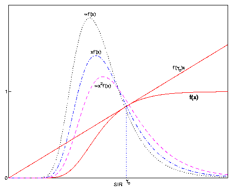
At the core of our analysis is a frame-success function (FSF) that gives the probability that a data packet is received successfully in terms of the terminal's received signal-to-interference ratio (SIR). This function is determined by physical attributes of the system, such as the modulation technique, the forward error detection scheme, the nature of the channel, and properties of the receiver. We do not impose any particular algebraic functional form (``equation'') on the FSF. Rather, we assume that all that is known about this function is that its graph is a smooth S-shaped curve, as displayed in fig.  (1), and base our analysis on properties derived from this shape. Hence, our analysis should apply to many physical layer configurations of practical interest. Reference [4] discusses further this modeling approach.

Below, we first build a relatively simple optimization model relevant to uplink data transmission in one VSG-CDMA cell. Afterward, we provide an outline of the general solution procedure. Then, we apply this procedure to the dual class situation of interest. Finally, we discuss our results, and comment on future relevant research.

2  General Formulation

2.1  Problem Statement

We seek to solve:

Maximize N å i=1  biTi(Gi,ai)

(1)

subject to

N å i=1  ai 1+ai =1

(2)

Gi ³ G0     i Î {1,¼,N}

(3)

In this simple model,

1. N is the number of terminals.
2. The throughput of terminal i is defined as R_CT_i(G_i,a_i), with
   

   Ti(Gi,ai):= f(Giai) Gi

   (4)

3. G_i=R_C/R_i, i Î { 1,¼,N} is the spreading gain of terminal i; i.e., the ratio of the channel's chip rate , R_C to the terminal's data transmission rate R_i (bits per second). G₀ ³ 1 is the lowest available spreading gain (determined by the highest available data rate).
4. a_i is the carrier-to-interference ratio (CIR) of the signal from terminal i received at the base station. a_i is defined as,
   

   ai:= Pihi N å [( j=1) || (j ¹ i)]  Pjhj+s2 = Qi N å [( j=1) || (j ¹ i)]  Qj+s2

   (5)

   with P_i the transmission power of terminal i, h_i its the path gain coefficient, h_iP_i:=Q_i its received power, and s² a representative of the average noise power and, possibly, out-of-cell interference. It can be shown that, with s²=0, the CIR's must be such that åa_i/(1+a_i)=1 (constraint (2)) to ensure feasibility [5].
5. The product G_ia_i , denoted as g_i , is terminal i's signal to interference (SIR) ratio.
6. b_i ³ 1 is a weight, which admits various practical interpretations. With no loss of generality, we can always set 1=b₁ £ ¼ £ b_N. In this work, we consider the special case in which 1=b₁=¼ = b_N1 and b = b_N1+1=¼ = b_N1+N2 with N₁+N₂=N. Thus, there are N₁ ``light weight'' terminals and N<sub>2</sub> ``important'' ones. However, in the development we often leave the weights expressed as b₁,¼,b_N to show the patterns. Initially, we take N₂=1, but later we discuss a generalization.
7. We assume that there is a frame-success function (FSF), f_S, which gives the probability of the correct reception of a data packet in terms of the received SIR. We assume that this function is such that f(x):=f_S(x)-f_S(0) has the general properties of the generalized ``S-curve'' introduced in [6] (see fig. (1)), and that it has a continuous second derivative. Becausef_S(0) is very small, the difference between f_S and f is generally negligible. Nevertheless, we have good technical reasons to make this correction, on the basis of [4]. No actual function is used, except to provide numerical examples.

In the development below, an asterisk used as a superscript on a variable denotes a specific value of the variable which satisfies certain optimality condition. We refer to terminals operating at maximal data rate as ``favored'' or ``favorite'', and call those terminals in the high-weight class ``important'', as opposed to ``ordinary''.

2.2  General solution procedure

The general procedure is as follows:

• Create an ``augmented'' objective function, combining the original objective function with Lagrange multipliers and the constraint equations
• Set up the first-order necessary optimizing conditions (FONOC). This involves setting the partial derivative of the augmented objective function with respect to each variable equal to zero. Moreover, inequalities of the form G₀-G_i £ 0 contribute equations of the form m_i(G₀-G_i)=0, where m_i is a Lagrange multiplier.
• Solve FONOC. Evidently, each equation of the form m_i(G₀-G_i)=0 requires that if G_i > G₀ , m_i be equal to zero; and that if m_i ¹ 0, G_i equal G₀. Both possibilities must be considered separately while finding various solutions to FONOC.
• A solution to FONOC provides a candidate for a maximizer. The second-order sufficient conditions may confirm the candidate as a maximizer. This maximizer may not be global.

3  Applying the General Solution Procedure

3.1  Augmented objective function

The ``augmented'' objective function is f(G₁,¼,G_N,a₁,¼,a_N)=

N å i=1  biTi(Gi,ai)+l æ ç è N å i=1  ai 1+ai -1 ö ÷ ø + N å i=1  mi(G0-Gi)

(7)

3.2  General First-Order Necessary Optimizing Conditions (FONOC)

The general FONOC can be expressed in vector form, with g_i=G_ia_i, as:

é ê ê ê ê ê ê ê ê ë b1¶T1(G1,a1)/¶G1-m1 : bN¶TN(GN,aN)/¶GN-mN b1f¢(g1)+l(1+a1)-2 : bNf¢(gN)+l(1+aN)-2 ù ú ú ú ú ú ú ú ú û = é ê ê ê ê ê ê ê ê ë 0 : 0 0 : 0 ù ú ú ú ú ú ú ú ú û

(8)

with ì ï ï ï í ï ï ï î N å i=1  (1+ai)-1=N-1 m1(G0-G1)=0 : mN(G0-GN)=0

(9)

Notice that

¶Ti(Gi,ai) ¶Gi = gif¢(gi)-f(gi) Gi2

(10)

3.3  Solving FONOC

3.3.1  Interior solution

It is natural to start by seeking an ``interior'' solution to FONOC, in which each G<sub>i</sub> is greater than G<sub>0</sub>, which requires m<sub>i</sub>=0, (see equations (9)). In [8] we discuss that, if G<sub>0</sub> is not ``too large'', one such solution exists and can be described by a closed-form expression.

In this solution, all terminals operate at an SIR value obtained by solving an equation of the general form:

xf¢(x)=f(x)

(11)

Reference [6] shows that for the class of generalized sigmoidal functions, such as f, there is a unique positive value g₀ which satisfies eq. (11). This value can be graphically identified in figure (1) as the abscissa of the point where the graph of f is tangent to a ray emanating from the origin; that is, tangent to the straight line y=f¢(g₀)x. Thus, if the function f is known, g₀ can be easily obtained graphically or eq. (11) can be solved numerically. For instance, g₀=10.75 and f(g₀)=0.83 for the FSF corresponding, under suitable assumptions, to non-coherent FSK with packet size M=80, which is

fs(x)= é ê ë 1- 1 2 exp æ ç è - x 2 ö ÷ ø ù ú û 80

(12)

However, the second-order optimality conditions reveal that this solution is always a ``saddle point'' (neither a maximizer nor a minimizer).

3.3.2   Single-Favorite Boundary Solution (SFBS)

The fact that the interior solution to FONOC is neither a maximizer, nor a minimizer indicates that the true maximizer is a solution in which one or more terminals operate at the lowest available spreading gain. We start by seeking an allocation satisfying FONOC in which only the spreading gain of the ``important'' terminal is set at the lowest available value, G₀ (i.e. this terminal operates at the highest available data rate), with other terminals' spreading gains to be determined by the analysis.

In [8], we fully discuss this case, for the general situation in which there is a distinct weight for each terminal. Our analysis shows that in order for this single-favorite solution to exist, the SIR of the ``non-favored'' terminals should be the previously mentioned g<sub>0</sub>, and the SIR of the favorite terminal should be a solution to the equation (C<sub>1</sub>x/G<sub>0</sub>+D<sub>1</sub>)<sup>2</sup>f¢(x)/f¢(g<sub>0</sub>)=1/b<sub>N</sub>. In this equation, C<sub>1</sub> and D<sub>1</sub> are constants which are largest when the weights of the non-favored terminals are smallest, and the other symbols are as previously defined. But the graph of the function (C<sub>1</sub>x/G<sub>0</sub>+D<sub>1</sub>)<sup>2</sup>f¢(x)/f¢(g<sub>0</sub>) has the same ``bell-shape'' of that of the function x²f¢(x) in fig. (1). Thus, the sought solution may not exist, because if G₀ is ``very large'', the peak of this function may fall below 1/b<sub>N</sub>, unless b<sub>N</sub> is also ``very large''. This makes intuitive sense, because when G₀ is ``very large'', the highest available data rate is relatively small, and keeping only one terminal operating at maximal data rate is not appealing, unless that terminal has ``a lot of weight''. However, when the highest available data rate is very high, an allocation in which only one terminal operates at this rate is more appealing.

3.3.3  Dual-Favorite Boundary Solution (DFBS) to FONOC

The ``single favorite'' boundary solution to FONOC may not exist, and even if it does exist, it may not lead to a global maximizer. We now seek an allocation satisfying FONOC, in which both the ``important'' terminal N, and the terminal whose index is N-1 (``sub-favorite'') operate at the highest permissible data rate. Below, we set G_N=G_N-1=G₀, and m_i=0 for 1 £ i £ N-2, and seek a solution to FONOC satisfying these hypotheses.

3.3.3.1  General structure of the solution  

Working with the first N-2 rows of the vector equation (8), and keeping in mind that our presumptions require that m_i=0 for 1 £ i £ N-2, we obtain

gi*=Gi*ai*=g0 for 1 £ i £ N-2

(13)

with g₀ defined as the unique positive solution to equation (11).

We also establish by working with the bottom half of the vector equation (8) that:

-l = bif¢(Gi*ai*)(1+ai*)2 for 1 £ i £ N-2

(14)

and

-l = bif¢(G0ai*)(1+ai*)2for N-1 £ i £ N

(15)

Combining equations (13) and (14), and the fact that b_i=1 for 1 £ i £ N-1, we obtain

ai*=aj* for 1 £ i , j £ N-2

(16)

Now, the constraint relation (6) ( å_i(1+a_i)^-1=N-1) becomes an equation with only three unknowns, a₁ , a_N-1 and a_N. Substituting eq. (16) into (6) yields, with x:=G₀a_N^* and y:=G₀a_N-1^*

N-2 1+a1 + 1 1+ y G0 + 1 1+ x G0 =N-1

(17)

Equations (14) and (15) imply that

f¢(y) æ ç è 1+ y G0 ö ÷ ø 2   = bf¢(x) æ ç è 1+ x G0 ö ÷ ø 2   (18) bf¢(x) æ ç è 1+ x G0 ö ÷ ø 2   = f¢(g0)(1+a1*)2 (19)

Equation (19) provides a closed-form expression for a₁^* in terms of x:

a1*= æ ç è 1+ x G0 ö ÷ ø   æ  ú Ö bf¢(x) f¢(g0)   -1

(20)

The function on the right-hand side of eq. (20) takes on values as low as -1, and yields a bell-shaped graph (such as that shown at the top of fig. (2)). But, physically, a₁ cannot be negative. Thus, the existence of a DFBS in which all the ordinary terminals are active necessitates that the SIR of the favorite terminal be held within certain range. This range expands as b grows, but shrinks as G₀ increases. Within this range, eq. (20) allows us to write eq. (17) as :

1 1+ y G0 + N-2 æ ç è 1+ x G0 ö ÷ ø   æ  ú Ö bf¢(x) f¢(g0)   + 1 1+ x G0 =N-1

(21)

Equation (18) cannot be solved explicitly. However, equations (18) and (21) form a system of two non-linear equations in two unknowns which is, in principle, solvable. Once we know the appropriate values of x^* and y^*, we can find a₁^*, the optimal CIR for terminals 1¼N-2, from eq. (20), and the corresponding spreading gain, from eq. (13), as g₀/a₁^*. Thus, from x^* and y^* we can obtain a complete dual-favorite solution to FONOC. Below, we describe this solution, and comment on its optimality.

3.3.3.2  Description of the DFBS to FONOC  

Figure (2) summarizes much of what can be said about the DFBS. For convenience, let h(t):=f¢(t)(1+t/G₀)², with t a ``dummy'' variable. The SIR's of the two terminals operating at maximal bit rate, denoted as x and y, must satisfy eq. (18) in order to satisfy FONOC. For the class of functions being considered, the graph of h(t) is ``bell-shaped'', as displayed in the top sub-figure of fig. (2). That is, there is exactly one point t^* at which this function has a global maximum, and for every t₁ £ t^* there is a t₂ ³ t^* such that h(t₁)=h(t₂). Thus, for every pair (x₂,y₂) which satisfies eq. (18), with x₂ ³ t^* and y₂ ³ t^*, there is a corresponding pair (x₁,y₁), with x₁ £ t^* and y₁ £ t^*, which also satisfies this equation, and so do (x₁,y₂), and (x₂,y₁).

For a given value of x, there are two values of y which satisfy bh(x)=h(y), unless x is ``too close'' to t<sup>*</sup>. The bottom sub-figure shows the ``X-shaped'' graph arising when we plot all points (x,y) satisfying this equation. For a fixed b, this graph has four distinct branches. The NE branch corresponds to points like (x₂,y₂) (top sub-figure), which are both to the right of the peak of h(t). Analogously, the NW, SW and SE branches correspond to points like (x₁,y₂) , (x₁,y₁) and (x₂,y₁) respectively.

The ``U-shaped'' curves at the bottom of fig. (2) are obtained by plotting the constraint equation (21) for various values of G₀ and a given b. But recall that eq. (21) is valid only for certain range of x. The points at which the U-curve (corresponding to the given values of G₀ and b) intersects the corresponding X-curve satisfy both equations (18) and (21), and hence each lead directly to a feasible solution to FONOC.

Increasing b has the effect of ``pulling apart'' the X-graph, and ``widening'' the U-curve. Thus, if these graphs intersect for a given b they still intersect after a moderate increase in b. On the other hand, the U-curve ``moves up'' when G₀ increases, while the X-graph is barely sensitive to changes in G₀. Thus, for G₀ large enough, no intersection (solution) exists. Otherwise, there are four intersection points, one in each of the branches of the concerned X-curve.

We are tempted to prefer the intersection point in the NE branch, where both x (the SIR of the favorite terminal) and y (the SIR of the sub-favorite) are as high as possible. But we must also consider the non-favored terminals, whose SIR is g₀, by eq. (13). The throughput of each non-favored terminal is obtained as f(g₀)/G₁=f(g₀)/(g₀/a₁^*) µ a₁^*. a₁^* is obtained from x^* through eq. (20), which gives rise to a ``bell shaped'' graph (see comments immediately following eq. (20)). Thus, a₁^* (and hence the throughput of the non-favored terminals) is decreasing in x^* beyond a certain value of x^*. Therefore, with possibly many non-favored terminals, it is not obvious that, of the four intersecting points, the one in the NE branch of the X curve leads to the greatest weighted throughput; however, this point does seem the best candidate. This issue merits further research.

4  Extension and Discussion

We have investigated the optimal power levels and data rates for terminals transmitting to one base station, in a scenario relevant to 3G CDMA. The objective function is the weighted sum of each terminal's throughput. Two weights, which admit various interpretations, including levels of importance, ``utilities'', or monetary prices, are considered. We have utilized a model which can accommodate many physical layer configurations of practical interest. The properties of the physical layer are embodied in the frame success function (FSF), which gives, in terms of received signal-to-interference ratio (SIR), the probability that a data packet is correctly received. Each physical layer has a preferred SIR, g₀, easily identified in the graph of the FSF.

Much of the preceding development has focused on the ``dual-favorite'' boundary solution (DFBS) to the first-order necessary optimizing conditions (FONOC), in which an ``important'' and an ``ordinary'' terminal operate at maximal data rate, while other terminals operate at certain optimal SIR, g<sub>0</sub>. This development can be extended to the more general multi-favorite case, in which all the ``important'' terminals, N₂, and several ``ordinary'' terminals, say n₁ £ N₁, operate at maximal data rate.

The key to obtaining the DFBS is to find a solution to a system of two non-linear equations in two unknowns, (18) and (21), in which the 2 variables are the SIR of the favorite and sub-favorite terminals. Through fig. (2), we described the solution to this system as one of the intersection points of the X-shaped graph (from eq. (18)) with the U-shaped graph (from eq. (21)). In the multi-favorite situation, eq. (18), bh(x)=h(y), would apply unmodified, with the understanding that x is the common SIR of all important terminals, and y is the common SIR of all the ordinary terminals operating at maximal data rate. The ``non-favored'' terminals would again operate with an SIR of g₀. But eq. (21) would need to be modified slightly as

n1 1+ y G0 + N1-n1 æ ç è 1+ x G0 ö ÷ ø   æ  ú Ö bf¢(x) f¢(g0)   + N2 1+ x G0 =N1+N2-1

(22)

The graph of eq. (22) has the same U-shape as that of eq. (21), and is appropriate over a certain range of x as discussed following eq. (20). Therefore, the general discussion summarized in the caption of fig. (2) still applies.

In principle, we would like n₁, the number of ``ordinary'' terminals operating at maximal data rate, to be as large as possible. However, the U-curve ``moves up'' when n₁increases. Thus, for sufficiently large n₁, the sought intersection may not exist. Moreover, when we make n₁=N₁ so that all terminals operate at maximal data rate, then the U-curve is replaced by a hyperbolic ``L-curve'', as displayed in fig. (2). For sufficiently low G<sub>0</sub>, the L-curve may intersect only the SW leg of the X-curve, in which both x and y are ``low'', and this would lead to a minimum, not a maximum.

More research is needed before we fully comprehend all interesting aspects of this problem. This includes performing various technical tasks, such as formally proving the shapes of some key graphs, and verifying certain second-order optimality conditions. The issues of QoS requirements, fairness, non-negligible out-of-cell interference, and decentralized implementations are of practical importance and deserve future consideration.

Acknowledgment

Supported in part by the NSF through the grant ``Multimodal Collaboration Across Wired and Wireless Networks'', and by NYSTAR through WICAT (http://wicat.poly.edu). Comments by Zory Marantz are gratefully acknowledged.

References

[1]

I, Chih-Lin and K.K. Sabnani, ``Variable spreading gain CDMA with adaptive control for true packet switching wireless network'', IEEE ICC, pp: 725 -730 vol.2, 1995

[2]

Lee, J.W., R.R. Mazumdar and N.B. Shroff, ``Joint Power and Data Rate Allocation for the Downlink in Multi-class CDMA Wireless Networks'', Proc. of 40th Allerton Conf. on Comm., Control and Comp., Oct. 2002

[3]

Ottosson, T. , and A. Svensson, ``Multi-rate schemes in DS/CDMA systems'', IEEE Vehicular Tech. Conf. , pp: 1006 -1010, vol.2, 1995

[4]

Rodriguez, V., ``Robust Modeling and Analysis for Wireless Data Resource Management'' To appear, IEEE WCNC, 2003

[5]

Rodriguez, V., ``From Power Levels to Power Ratios and Back: A Change of Domain and its Modeling Implications'', WICAT Tech. Rep. 02-011, Polytechnic Univ., 2002
http://wicat.poly.edu/reports

[6]

Rodriguez, V., ``Maximizing the Ratio of a Generalized Sigmoid to its Argument'', WICAT Tech. Rep. 02-010, Polytechnic University, 2002
http://wicat.poly.edu/reports

[7]

Rodriguez, V., and D.J. Goodman ``Prioritized Throughput Maximization via Rate and Power Control for 3G CDMA: The 2 Terminal Scenario'', Proc. of 40th Allerton Conf. on Comm., Control and Comp., Oct. 2002

[8]

Rodriguez, V., and D.J. Goodman, ``Power and Data Rate Assignment for Maximal Weighted Throughput in 3G CDMA'' To appear, IEEE WCNC, 2003

[9]

C. W. Sung and W. S. Wong, ``Power Control and Rate Management for Wireless Multimedia CDMA Systems'', IEEE Trans. Commun., vol. 49, no. 7, pp. 1215-26, July 2002

[10]

Ulukus, S. and L.J. Greenstein ``Throughput maximization in CDMA uplinks using adaptive spreading and power control'' IEEE ISSSTA 2000, pp: 565 -569 vol.2